Chapter 1: Introduction #

We see... that the theory of probabilities is at bottom nothing but common sense reduced to calculus: it enables us to appreciate with exactitude that which excellent minds sense by a kind of instinct for which they are often unable to account.

— Pierre-Simon Laplace

To count is a modern practice, the ancient method was to guess...

— Samuel Johnson

These notes provide tools to study combinatorial objects, also called discrete structures, which are collections of objects that can be decomposed into discrete parts. Because this definition is so general, our techniques find application across a wide variety of areas, like computer science, mathematics, the natural sciences, linguistics, and even the textile arts. We use tools from pure mathematics to study concrete problems, with a focus on effective methods that can be implemented on a computer.

This first chapter gives a high-level view of our goals and approach. In order to illustrate the breadth of applications for combinatorial enumeration we introduce a large variety of objects without giving full definitions, and give a number of references for those wanting additional details. The important combinatorial objects that will be studied in the rest of these notes will be introduced in detail in Chapter 2.

Combinatorial Sequences #

We study the behaviour of combinatorial objects using sequences. Our sequences can have complex number values, although since we are typically counting things they usually take values in the natural numbers $\mathbb{N}=\{0,1,2,\dots\}.$

A one-dimensional sequence $(a_n)$ can be viewed as an infinite list $$(a_n) = a_0,a_1,a_2,\dots$$ of complex numbers, although formally it is a map that takes a number $n \in \mathbb{N}$ and assigns it a value $a_n \in \mathbb{C}.$ Similarly, a $d$-dimensional sequence $(a_{\mathbf{n}})$ is a map that takes a vector $\mathbf{n}\in\mathbb{N}^d$ and assigns it a value $a_{\mathbf{n}}\in\mathbb{C}.$

Such a sequence might

count the number of objects in a combinatorial class

Example: $c_n$ is the number of ways to make change for $n$ dollars using pennies, nickels, dimes, and quarters
capture the probability that an event occurs

Example: $p_n$ is the probability that two numbers in $\{1,\dots,n\}$ are coprime
track the complexity cost of an algorithm

Example: $q_n$ is the average number of comparisons performed by quicksort on all permutations of $1,\dots,n$
encode a combinatorial class with parameters

Example: $b_{k,n}$ is the number of binary trees on $n$ nodes with $k$ leaves

Our goal is to take a collection of combinatorial objects, capture their behaviour using a sequence, and then say something interesting.

Properties of Sequences #

Here are some of the interesting things we might be able to determine.

1. Explicit Formulas #

In order to manipulate sequences, by hand or on a computer, we need some way of representing them. Many combinatorial sequences admit explicit formulas, meaning a general term $a_n$ can be written as a nice expression in $n.$

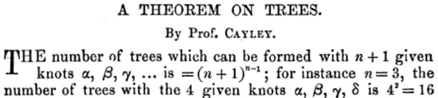
Example: In 1860 Borchardt [Bo60] discovered the formula $(n+1)^{n-1}$ for the number of labeled trees with $n+1$ vertices, a result popularized and extended in an 1889 article of Cayley [Ca89]. We will discuss three proofs of this classic result, using bijections, generating functions, and determinants.

Figure: The start of Cayley’s 1889 article.

The precise meaning of a nice (or even non-trivial) expression can be surprisingly hard to pin down. Roughly speaking, we want to avoid situations like the following.

Non-Example: If $a_n$ counts the elements in a set $\mathcal{A}_n$ then we can always write $a_n = \sum_{\alpha\in\mathcal{A}_n} 1.$ Of course, this tells us nothing interesting.

One of the more interesting approaches to classifying nice formulas is to treat them from a complexity perspective, so that a polynomial-time formula for a sequence that grows exponentially is nice, but a quadratic-time formula for a sequence that grows linearly is not nice. It is also possible to ask for the most efficient formula possible for a given sequence.

Example: Let $g_n$ denote the number of (non-isomorphic simple) graphs on $n$ vertices. In 1982 Wilf [Wi82] asked whether $g_n$ can be computed in polynomial time with respect to $n,$ and this problem is still open 40 years later.

We won’t consider this meta-question any further: nice expressions for us will typically involve only the usual arithmetic operations, exponentials, factorials, binomial coefficients, and (a small amount of) definite summation with explicit bounds. More information about classifying nice formulas can be found in [Wi82] and [Pa18] .

2. Encodings #

When a sequence doesn’t have a simple explicit expression, or we don’t know how to find one, we need another way of encoding it. Many sequences can be implicitly encoded by recurrence relations, where a general term $a_n$ is related to previous terms. Two common types of sequences that appear often in combinatorics are the following.

A C-finite sequence satisfies a linear recurrence with constant coefficients.

Example: The Virahanka-Fibonacci sequence $(v_n)$ is defined recursively by $v_0=v_1=1$ and $v_{n+2} = v_{n+1} + v_n$ for all $n \geq 0.$
A P-recursive sequence satisfies a linear recurrence with polynomial coefficients.

Example: If $r_n$ denotes the number of ways to place $n$ pieces on an $n\times n$ board such that no two pieces lie in the same row or the same column then we can define the initial condition $r_0=1$ and show that $$r_{n+1} = (n+1)r_n$$ for all $n \geq 0$ (can you see why?). In this case we can simply solve the recurrence to obtain $$r_n = n(n-1)(n-2)\cdots(2)(1)=n!$$

If $d_n$ denotes the number of ways to place $n$ pieces on an $n\times n$ board such that no two pieces lie in the same row or the same column and no piece lies on the diagonal then $d_0=1$ and $d_1=0,$ while $$d_{n+2} = (n+1)d_{n+1} + (n+1)d_n$$ for all $n \geq 0$ (can you see why?). We will see expressions for $d_n$ in later chapters.

Remark: Both $r_n$ and $d_n$ are examples of non-attacking rook sequences, which enumerate the number of ways to place non-attacking rooks on chess boards with certain squares removed. The enumeration of non-attacking rook patterns was popularized in classical recreational mathematics like Dudeney’s 1917 book Amusements in Mathematics [Du17] but has received modern research attention from communities interested in the study of certain types of permutations. Counting non-attacking rook sequences is also equivalent to computing the so-called permanent of matrices with 0 and 1 entries, which is (most likely) very difficult in general. Non-attacking sequences for other chess pieces are also well-studied.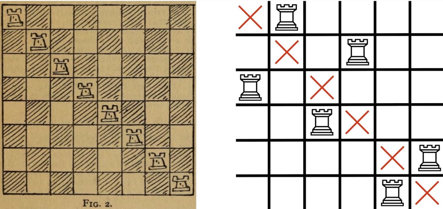

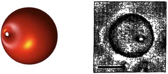
Figure: (Left) A figure from Amusements in Mathematics. (Right) A non-attacking rook pattern with no rooks on the diagonal.

Example: Developing and verifying an accurate way to predict the shape of biomembranes like blood cells is an important problem in biology and applied geometry. The influential Canham-Helfrich model states that after fixing the genus (number of holes), area, and volume of a biomembrane then its shape is determined by minimizing a certain energy function. Recently, Yu and Chen [YuCh22] reduced the problem of proving that the model has a geometrically unique solution for a large collection of genus one surfaces to proving that a P-recursive sequence $(c_n)$ encoded by initial conditions and an explicit P-recurrence $$ r_7(n)c_{n+7} + \cdots + r_0(n)c_n = 0 $$ contains strictly positive terms. Melczer and Mezzarobba [MeMe22] proved this positivity using techniques from computer algebra and asymptotic combinatorics.

(Left) Shape of a genus one membrane predicted by the Canham-Helfrich model (figure from Yu and Chen). (Right) A genus one biomembrane observed under a microscope (figure from Michalet and Bensimon).

We can view recurrences satisfied by combinatorial sequences as data structures that help us enumerate combinatorial objects. Perhaps the most crucial observation for enumerative combinatorics is that instead of encoding a sequence directly, it is often much more useful to encode a series that it generates.

The generating series or generating function of a univariate sequence $(a_n)=a_0,a_1,\dots$ in the variable $z$ is the series

$$ A(z) = \sum_{n=0}^{\infty} a_nz^n . $$

The generating series is a formal series: we do not worry (at this point) about when the series converges. We go into detail on formal series and generating series in Chapter 4.

Generating functions are useful because series have a natural algebraic structure that neatly expresses common relationships between combinatorial objects. Although one could define a similar structure directly in terms of sequences, these relationships are more straightforward in terms of series.

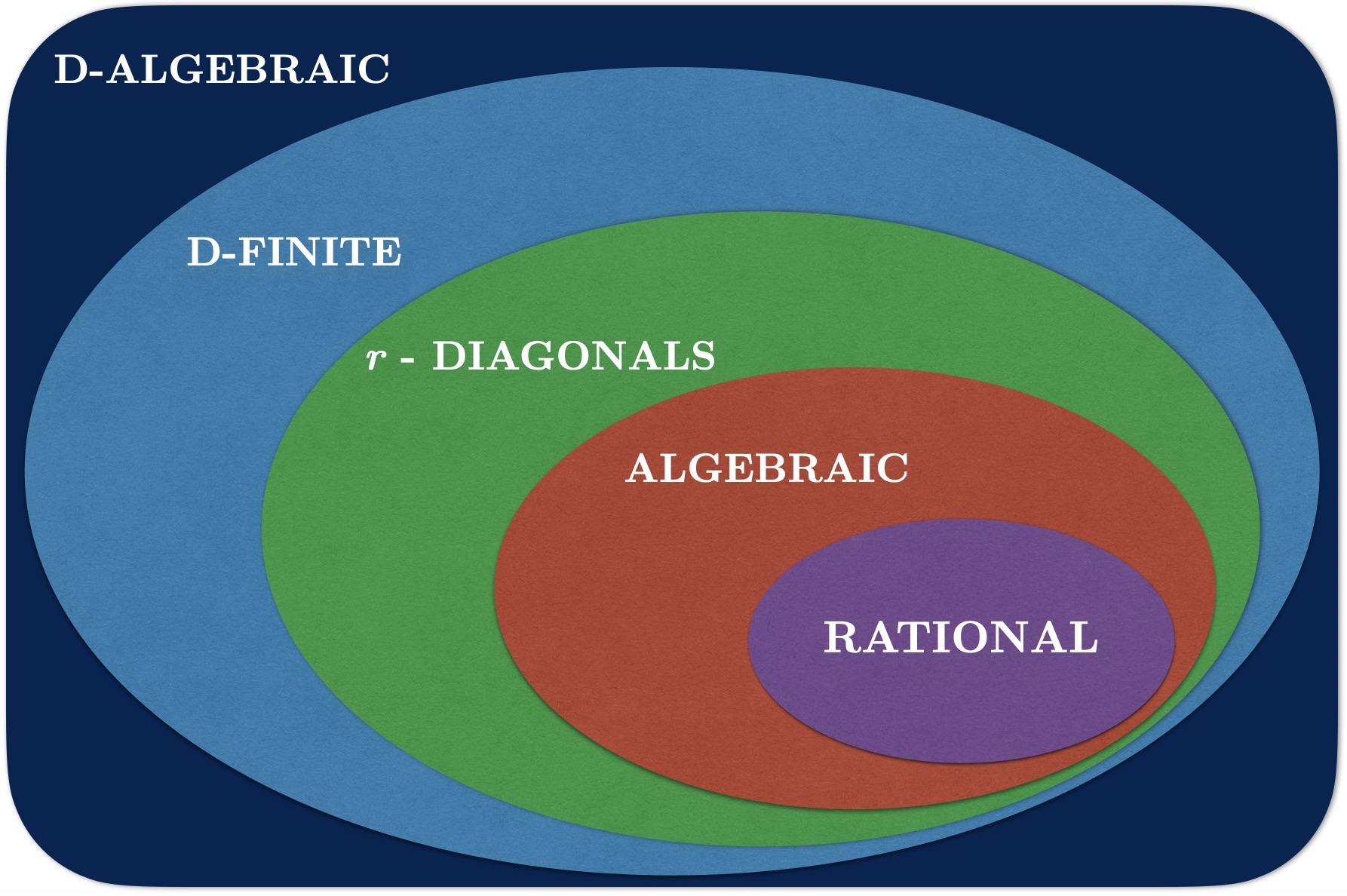
Many combinatorial generating series are naturally encoded by different algebraic and differential equations. For instance,

A rational series can be encoded by the polynomials defining its numerator and denominator.
Example: As we will see in Part 4 of these notes, any C-finite sequence has a rational generating series (and any sequence with a rational generating series is C-finite). For instance, the generating series $V(z)$ of the Virahanka-Fibonacci sequence $(v_n)$ is $$ V(z) = \frac{1}{1-z-z^2}. $$ We will discuss how to think of rational functions are formal series in Chapter 4 – for now we simply note that $(v_n)$ forms the coefficients of the Taylor series of $V(z)$ at the origin. For instance, running the Sage code
```
(1/(1-x-x^2)).series(x,6)
```
gives the series truncation
```
Out: 1 + 1*x + 2*x^2 + 3*x^3 + 5*x^4 + 8*x^5 + Order(x^6)
```
whose coefficients are $(v_0,\dots,v_5) = (1,1,2,3,5,8).$
An algebraic series $f(z)$ satisfies $P(z,f(z))=0$ for some polynomial $P(z,y) \in \mathbb{Z}[z,y].$ Such a series can be encoded by $P$ and a finite number of terms to specify it among the roots of $P.$

Example: The sequence of Catalan numbers $c_n = \frac{1}{n+1}\binom{2n}{n}$ has an incredible number of combinatorial interpretations: they form the longest entry in the Online Encyclopedia of Integer Sequences and Stanley [St15] lists 207 objects they enumerate. As we will see in later chapters, the generating series $C(z)$ of $(c_n)$ satisfies the polynomial equation $$ zC(z)^2 - C(z) + 1 = 0, $$ and we can write $$ C(z) = \frac{1-(1-4z)^{1/2}}{2z} $$ provided we either interpret $(1-4z)^{1/2}$ as a formal series using Newton’s binomial theorem or restrict $z$ to values where the generating series converges to this algebraic function (which turns out to be when $|z|<1/4$). Again, we will discuss the necessary background in Chapter 4.
A D-finite series satisfies a linear differential equation with polynomial coefficients, and can be encoded by such an equation together with initial conditions.

Example: Any P-recursive sequence has a D-finite generating series (and any sequence with a D-finite generating series is P-recursive). For instance, the non-attacking rook sequences $r_n$ and $d_n$ above have generating series $R(z)$ and $D(z)$ that satisfy $$ z^2D^\prime(z) - (1-z)D(z) + 1 = 0 $$ and $$ z^2(1+z)R^\prime(z) - (1-z)(1+z)R(z) + 1 = 0. $$
A D-algebraic series satisfies a polynomial differential equation with polynomial coefficients, and can be encoded by such an equation together with initial conditions.

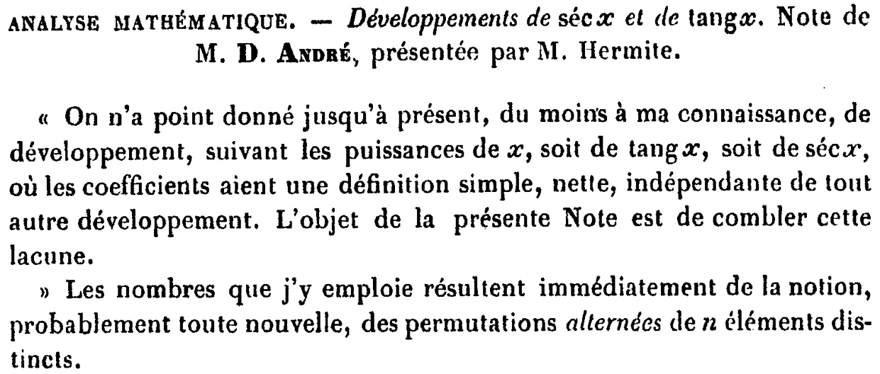
Example: An alternating permutation of size $n$ is an arrangement of the numbers $1,2,\dots,n$ with $n$ odd such that the first number is larger than the second, the second is smaller than the third, the third is larger than the fourth, and so on. If $a_n$ is the number of alternating permutations of size $n$ (equal to zero if $n$ is even) then André [An79] proved in 1879 that $\sum_{n \geq 0}\frac{z^n}{n!} = \tan z$ (we will see why later). It can be shown that $y(z)=\tan z$ does not satisfy any linear differential equation, however the reader might remember the identity $$ y^\prime(z) = y(z)^2 + 1 $$ from calculus.

Figure: The start of Andre’s 1879 article.

Example: Duffin [Du81] showed that for any real continuous function $g(z)$ and accuracy target there exists a four times continuously differentiable solution of the polynomial differential equation $$ 2F^{\prime\prime\prime\prime}(z)F^\prime(z)^2 - 5F^{\prime\prime\prime}(z)F^{\prime\prime}(z)F^\prime(z) + 3F^{\prime\prime}(z)^3 = 0$$ which approximates $g(z)$ to the desired accuracy over the real numbers. Intuitively, this means that a polynomial differential equation satisfied by the generating series of a combinatorial family may not restrict the type of structure the combinatorial family has. Perhaps unsurprisingly in light of this, there are many undecidable properties of general D-algebraic series (for instance, checking whether their coefficients decay to zero or grow to infinity). Solving D-algebraic equations can also be used to simulate general Turing machines.

Determining a recurrence for a sequence, or an equation satisfied by its generating series, allows one to say something about the structure of the class, and is usually the first step towards determining the other properties discussed here.

Figure: Some increasingly complicated classes of generating series. The class of $r$-diagonals contains generating series defined in terms of multivariate rational series.

3. Fast Algorithms #

Often we can use the definition of a sequence, or one of the encodings discussed above, to create an algorithm allowing us to efficiently compute terms.

Let $(v_n)$ be the Virahanka-Fibonacci sequence and consider the following Sage code.
M = Matrix(ZZ,2,2,[1,1,1,0]) # matrix with rows [1,1] and [1,0]
def bin_pow(n):
	if n == 1:		return M
	elif n%2 == 0:	return bin_pow(n/2)^2
	else:			return bin_pow((n-1)/2)^2*M

def fib(n):			return add(bin_pow(n)[1])

timeit('fib(10^6)')	# compute v_(10^6)
Running this on a 2020 Macbook Pro gives the output
Out: 25 loops, best of 3: 10.1 ms per loop
which implies that we can compute the millionth Fibonacci number (having more than 200,000 decimal digits) in around 10 milliseconds. We will see later why the fib(n) function computes $v_n$ (although you might be able to figure it out for yourself if you try!) and how to generalize to other C-finite sequences.

This example illustrates how, for many sequences, we can almost instantly compute any specific terms needed in applications. However, such algorithms do not immediately help one determine the behaviour of sequences (although computing sequence terms is crucial for exploring or guessing behaviour).

4. Asymptotics #

Instead of focusing on exact formulas, or precise algorithms, it is often useful to focus on approximating large-scale behaviour. In Part 4 we will see techniques to approximate a sequence $(a_n)$ as $n$ gets large.

Given sequences $a_n$ and $b_n$ we say that $a_n$ and $b_n$ have the same dominant asymptotic behaviour and write $a_n \sim b_n$ whenever $a_n/b_n \rightarrow 1$ as $n\rightarrow\infty.$

Factorial

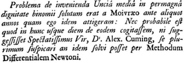
Although $n!$ has a simple definition, Stirling’s approximation $$ n! \sim (n/e)^n \sqrt{2\pi n} $$ from his 1730 text [St30] allows us to get a better handle on how the factorial behaves for large $n.$

Figure: Text from the preface of Stirling’s Methodus Differentialis (English translation: The problem about finding the middle coefficient in a very large power of the binomial had been solved by de Moivre some years before I considered it: And it is probable that to this very day I would not have thought about it, unless that most esteemed man, Mr Alex. Cuming, had not stated that he very much doubted that it could be solved by Newton’s Method of Differences.)

Partitions

If $p_n$ denotes the number of integer partitions of size $n$ then Hardy and Ramanujan [HaRa18] derived the asymptotic formula $$ p_n \sim \frac{\exp\left(\pi\sqrt{2n/3}\right)}{4n\sqrt{3}} $$ using analytic techniques (a result impressive enough to be a large plot point in a Hollywood movie). Although there is technically an explicit formula for $p_n,$ it took hundreds of years to discover and is extremely unwieldy.

Unlabelled Graphs

As noted above, it has been open since the 1980s whether the number $g_n$ of simple graphs on $n$ vertices can be computed in polynomial time. However, the asymptotic behaviour $$ g_n \sim \frac{2^{\binom{2n}{n}}}{n!} $$ follows from classical probabilistic work of Erdős and Rényi [ErRe63] which implies that as $n\rightarrow\infty$ the total number of unlabelled graphs approaches the number $2^{\binom{2n}{n}}$ of labelled graphs divided by the number $n!$ of ways to permute the labels.

Quadrant Walks

Let $w_n$ denote the number of ways to start at $(0,0)$ and take $n$ steps in $$\{(\pm1,0),(0,\pm1)\} = \{\text{North}, \text{South}, \text{East}, \text{West}\}$$ without ever being at a location with a negative coordinate. Walk models like this are used in queuing theory to model objects entering and being processed from lines, since there can never be a negative number of objects in lines. In addition to combinatorial techniques, probabilistic methods are powerful tools for such problems since the probability $p_n$ that a uniform random walk of length $n$ stays in the first quadrant satisfies $p_n = w_n/4^n.$

Animation (click to start/stop): 400 random walks of length 300. Walks go transparent as they leave the first quadrant, and only one walk stays in the first quadrant for all 300 steps. The probability $p_{300}=w_{300}/4^{300}$ that a uniform random walk of length 300 stays in the quadrant is a large rational number equal to $0.00422\dots$ In fact, as $n$ goes to infinity it can be shown that the probability that a walk of length $n$ stays in the first quadrant gets closer and closer to $4/\pi n$ (when $n=300$ this approximation is $0.00424\dots$).

Quicksort

Quicksort is an extremely popular algorithm that sorts a list of unique numbers by picking an element (called a pivot) of the list, dividing the list into the elements that are smaller than the pivot and the elements that are larger than the pivot, and then recursively sorting these two sublists. If $c_n$ denotes the average number of comparisons performed by quicksort on all permutations of $\{1,\dots,n\}$ then we will prove $$ c_n = 2(n+1) \sum_{k=1}^n \frac{1}{k} - 4n, $$ an explicit expression but not one that easily shows the behaviour of quicksort’s runtime. In fact, we will also prove $ \sum_{k=1}^n \frac{1}{k} \sim \log n$ so $$c_n \sim 2n\log n.$$

5. Limit Theorems #

Perhaps the most striking large-scale results are limit theorems for combinatorial objects with parameters. Most commonly, we examine the behaviour of terms in a multivariate sequence when one index is fixed and large. In light of the central limit theorem, it might not be surprising that many parameters in combinatorial classes exhibit Gaussian/normal behaviour as the size of the objects goes to infinity.

Animation (click to start/stop): This animation shows the cumulative results of counting the divisions performed by the Euclidean algorithm on 2001 random polynomial pairs $(f,g)$ over the finite field of order three with $f$ monic and $\deg g < \deg f = 500.$ Because the set of polynomials of fixed degree whose coefficients come from a finite field form a finite set of discrete objects, the techniques of enumerative combinatorics can be used to show that the number of divisions approximates a limiting normal curve.

Tables 1 and 2 of [Hw22] list 26 limit laws proven by the late Philippe Flajolet for various combinatorial objects, including patterns in words, cost analyses of various sorting algorithms, parameters in different kinds of trees, polynomials with restricted coefficients, and ball-urn models.

Although we will not prove limit theorems in these notes, we will see techniques to characterize multivariate generating series and find the mean and variance of combinatorial parameters (usually an important step towards establishing limit theorems).

Summary #

This Chapter is meant to give an enticing overview to some of the techniques of enumeration, and the problems we can address with them. We hope this whirlwind presentation has piqued the reader’s interest, and is the start of a fulfilling journey into the rich wonders of enumerative combinatorics.