Chapter 2: Combinatorial Classes #

The interplay between generality and individuality, deduction and construction, logic and imagination – this is the profound essence of live mathematics... In brief, the flight into abstract generality must start from and return again to the concrete and specific.

— Richard Courant

To many, mathematics is a collection of theorems. For me, mathematics is a collection of examples; a theorem is a statement about a collection of examples and the purpose of proving theorems is to classify and explain the examples...

— John B. Conway

In this chapter we formalize our study of combinatorial objects, and discuss some interesting applications of different combinatorial families. Our discussion starts with the following definition.

A combinatorial class consists of a set of objects $\mathcal{C}$ together with a weight function $w:\mathcal{C}\rightarrow\N$ (also known as a size function) such that for any $n\in\mathbb{N}$ the set $$\mathcal{C}_n = \{\sigma \in \mathcal{C} : w(\sigma) = n\}$$ containing the elements of weight $n$ is finite (i.e., there are a finite number of objects of any weight). A subclass of a class $(\mathcal{C},w)$ is any class whose objects form a subset of $\mathcal{C}$ and whose weight function is still $w.$

Note that although there must be a finite number of objects of any weight, the set $\mathcal{C}$ itself can be (and usually is) infinite.

Example: Let $\mathcal{C}=\{\epsilon,0,1,00,01,10,11,\dots\}$ be the set of all finite length sequences of $0$s and $1$s, where $\epsilon$ denotes the empty sequence (containing no terms). There are many possible choices of weight function, some of which make $\mathcal{C}$ a combinatorial class and some of which don’t. For example, if $$w(s) = \text{length of $s$}$$ then $\mathcal{C}$ and $w$ define a combinatorial class.

On the other hand, if $$w(s) = \text{\# of zeroes in $s$}$$ then $\mathcal{C}$ and $w$ do not define a combinatorial class. For instance, this choice of $w$ gives an infinite number of elements $\epsilon,1,11,111,\dots$ with weight zero.

Exercise: Define two more weight functions $w$ that make the set $\mathcal{C}$ in the last example a combinatorial class. Then, define two more weight functions that do not make $\mathcal{C}$ a combinatorial class.

A combinatorial class is the minimal amount of structure needed for enumeration (a set of objects to study and a notion of weight/size). Once we have a combinatorial class, we can start to determine its properties.

If $\mathcal{C}$ is a combinatorial class then the counting sequence $(c_n)$ of $\mathcal{C}$ is the sequence where $c_n=|\mathcal{C}_n|$ equals the number of elements in $\mathcal{C}$ with weight $n.$ The generating function of $\mathcal{C}$ is the series $$ C(z) = \sum_{n \geq 0} c_nz^n. $$ We will discuss the mathematical background for such series and generating functions in Chapter 4.

Remark: Although the counting sequence and generating function both depend on the weight function, we omit it from our notation. It is convention to use a calligraphic letter for a combinatorial classes, the lower-case version of the letter for its counting sequence, and the upper-case version of the letter for its generating function. For instance, after fixing a weight function the combinatorial class $\mathcal{A}$ would have counting sequence $(a_n)$ and generating function $A(z).$

Example (continued): The combinatorial class $\mathcal{C}$ defined above for $0$ - $1$ sequences with weight given by length has counting sequence $c_n = 2^n$ and generating function $$ C(z) = \sum_{n \geq 0}2^nz^n. $$ In fact, we will see in Chapter 4 that this can be simplified as a formal geometric series, giving $$ C(z) = \frac{1}{1-2z}. $$ Note that the empty sequence $\epsilon$ gives a single element of size zero, allowing us to use one formula for all $n.$ We often add (or remove) objects of size zero from a combinatorial class to make a problem under consideration as simple as possible.

The goal of a univariate enumeration problem is to start with a description of a combinatorial class and its weight function, and say something interesting about the class, its counting sequence, or its generating function (in the manner discussed in Chapter 1). In Part 3 of these notes, where we discuss parameters, we will introduce weight functions that map to vectors.

With these formalities out of the way, we now survey a variety of combinatorial classes. Of course, this list is far from exhaustive: there are far too many beautiful and well-studied objects to list them all here, but we aim to illustrate the breadth and applicability of enumerative techniques and introduce the families we will return to most in these notes.

Strings #

Let $\Omega$ be a non-empty finite set. For any positive integer $n$ the words or strings of length $n$ over the alphabet $\Omega$ form the set $$ \Omega^n = \{ (w_1,\dots,w_n) : \text{ all } w_j \in \Omega \}$$ of tuples of length $n$ whose elements come from $\Omega,$ and we let $\Omega^0 = \{\epsilon\}$ be the set containing the empty string $\epsilon.$

The words or strings over the alphabet $\Omega$ form the set $$\Omega^* = \bigcup_{n \geq 0}\Omega^n$$ of all words of any length over the alphabet $\Omega$ (including the empty string). Unless otherwise specified, we make this set a combinatorial class by defining the weight of a word to be its length (although other weight functions are also possible).

Although the elements of $\Omega^{*}$ are tuples, we usually drop parentheses and write $w_1\cdots w_n$ for an element $(w_1,\dots,w_n).$

Example: If $\Omega=\{0,1\}$ then we call $\Omega^{*}$ the class of binary strings. This class was examined in the previous examples above.

Example: If $\Omega=\{A,C,G,T\}$ then $\Omega^{*}$ encodes possible DNA sequences. Note that actual human DNA sequences are made up of approximately 3 billion A/C/G/T characters (called nucleotides)!

Enumerating the combinatorial class $\mathcal{C} = \Omega^{*}$ is straightforward: an element of weight $n$ is defined by picking $n$ elements in $\Omega,$ so the counting sequence satisfies $c_n = |\Omega|^n$ and the generating function is always the geometric series $$ C(z) = \sum_{n \geq 0} |\Omega|^n z^n = \frac{1}{1-|\Omega|z}. $$

In practice, then, interesting string enumeration problems typically involve subclasses defined by an alphabet $\Omega$ and a subset of $\Omega^{*}$ defined by some restrictions.

Example: Let $\mathcal{F}$ be the combinatorial class consisting of all binary strings (i.e., elements of $\Omega^{*}$ with $\Omega=\{0,1\}$) that have no consecutive 1s. The elements of $\mathcal{F}$ can be listed in order of increasing weight, $$ \mathcal{F} = \{ \epsilon, 0, 1, 00, 01, 10, 000, 001, 010, 100, 101, \dots \}. $$ The combinatorial description of $\mathcal{F}$ allows us to determine a recurrence satisfied by its counting sequence $(f_n).$ Indeed, if $w \in \mathcal{F}$ has length $n \geq 2$ then either

• $w$ ends in a 0, meaning it can be uniquely decomposed as an element of $\mathcal{F}$ with length $n-1$ followed by a 0, or
• $w$ ends in a 1, meaning it can be uniquely decomposed as an element of $\mathcal{F}$ with length $n-2$ followed by a 01 (since there cannot be consecutive 1s).

This decomposition proves the recurrence relation $$ f_n = f_{n-1} + f_{n-2} \quad (n \geq 2)$$ and the initial conditions $f_0 = 1$ and $f_1 = 2$ can be determined by writing out the elements of $\mathcal{F},$ uniquely determining $(f_n).$ We will see general methods for solving linear recurrences such as this in Part 4 of these notes.

Any family of discrete structures can be encoded on a computer, and therefore can be described by some class of binary strings. Although this means any enumeration problem can be viewed as a string enumeration problem, it is often much more convenient to use a more specific combinatorial class, such as those described below. Studying a family of discrete objects through the lens of string enumeration can be worthwhile when the family is described as a collection of strings avoiding a certain pattern, or set of patterns (binary strings with no consecutive 1s, decimal numbers with no three even digits in a row, etc.).

Advanced Applications of String Enumeration #

Techniques studying patterns in strings with various properties find use in a huge number of areas. In addition to bioinformatics, some other applications include computational linguistics and forensic accounting.

Subsets and Permutations #

Let $\Omega$ be a finite set with $n$ elements. Recall that the subsets of $\Omega$ are the sets (including the empty set) whose elements come from $\Omega.$

Example: If $\Omega = {\big\{} 🍎, 😄, 🌈 {\big\}}$ then the subsets of $\Omega$ are the eight sets $$ \begin{aligned} {\Big\{}🍎, 😄, 🌈{\Big\}}& \qquad {\Big\{}😄, 🌈{\Big\}} \qquad {\Big\{}🍎, 🌈{\Big\}} \qquad {\Big\{}🍎, 😄{\Big\}} \\ &\;\;{\Big\{}🍎 {\Big\}} \qquad {\Big\{}😄 {\Big\}} \qquad {\Big\{}🌈 {\Big\}} \qquad \varnothing \end{aligned} $$

The permutations of $\Omega$ are the length $n$ tuples containing each element of $\Omega$ exactly once. For convenience, we often remove the commas between elements in the tuple, leaving spaces instead, and drop the surrounding parentheses (make sure you leave enough space to distinguish the elements of the permutation).

Example: If $\Omega = {\big\{} 🍎, 😄, 🌈 {\big\}}$ then the permutations of $\Omega$ are the six tuples $$ \begin{aligned} 🍎 \, 😄 \, 🌈 \qquad 🍎 \, 🌈 \, 😄 \qquad 😄 \, 🍎 \, 🌈 \\ 😄 \, 🌈 \, 🍎 \qquad 🌈 \, 🍎 \, 😄 \qquad 🌈 \, 😄 \, 🍎 \end{aligned} $$

Remark: The number of subsets and permutations of $\Omega$ depend only on the size of $\Omega,$ not which elements it contains. For instance, replacing 😄 by 😱 in the above examples gives an analogous (if slightly more terrifying) result. For this reason, we usually study subsets and permutations of the sets $[n] = \{1,2,\dots,n\}$ for $n\in\mathbb{N}.$

Fix a positive integer $N.$ The class $\mathcal{C}^{[N]}$ of subsets of $[N]$ consists of all subsets of $[N]$ with weight defined by the number of elements in the subset. Note that, unlike most of the combinatorial classes we are interested in, $\mathcal{C}^{[N]}$ contains only a finite number of elements.

Enumerating $\mathcal{C}^{[N]}$ is straightforward: there are $\binom{N}{k}$ ways to select $k$ elements of $[N]$ for a subset of size $k$ so $c^{[N]}_k = \binom{N}{k}$ and the generating function for this class is the polynomial $$ C^{[N]}(z) = \sum_{k=0}^N \binom{N}{k}z^k = (1+z)^N. $$ Typically, we consider subclasses of $\mathcal{C}^{[N]}$ defined by restrictions on the subsets that can appear.

The set $\mathcal{S}_n$ of permutations of length $n$ consists of the permutations of $[n]$ and the class of permutations $\mathcal{S}$ consists of all permutations of all lengths with the weight function mapping a permutation to its length.

It is common to use Greek letters like $\pi$ and $\sigma$ for elements in $\mathcal{S}.$ There are four common ways to view a permutation $\pi \in \mathcal{S}_n,$ all of which are equivalent.

• One-line Notation: The element $\pi$ is expressed as the tuple $\pi_1 \cdots \pi_n$ mentioned in the definition above.

• Two-line Notation: The element $\pi$ is expressed as a table with two rows. The first row contains the numbers $1,\dots,n$ in order and the second contains the tuple $\pi.$

  Example: The permutation $\pi = 3 \, 5 \, 4 \, 1 \, 2$ can be expressed by the table

  $i$	$1$	$2$	$3$	$4$	$5$
  $\pi_i$	$3$	$5$	$4$	$1$	$2$

• As a Function: The element $\pi$ is viewed as a function from $[n]$ to $[n]$ that takes $i\in [n]$ to the value $\pi_i\in [n].$

  Example (continued): The permutation $\pi = 3 \, 5 \, 4 \, 1 \, 2$ is equivalent to the function from $\{1,2,3\}$ to itself defined by $$ \pi(1) = 3, \quad \pi(2) = 5, \quad \pi(3)=4, \quad \pi(4)=1, \quad \pi(5)=2. $$

  Under this interpretation $\mathcal{S}_n$ contains all bijections from $[n]$ to itself, and therefore forms the permutation group of size $n$ (see Chapter 3 for more on bijections).

• Cycle Notation: If we consider $\pi$ as a function then we can start with $1$ and keep applying $\pi$ to get a sequence of numbers $1, \pi(1), \pi(\pi(1)),\dots.$ Because $\pi$ is a permutation, this sequence will eventually repeat, giving the cycle of $\pi$ containing 1. Repeating this with the other elements of $[n]$ allows us to break $\pi$ into disjoint cycles, which we write as consecutive tuples.

  Example (continued): Looking at the last example, we see that $\pi = 3 \, 5 \, 4 \, 1 \, 2$ maps $$1 \rightarrow 3 \rightarrow 4 \rightarrow 1$$ so $\pi$ has a cycle $(1 \, 3 \, 4).$ Since $2$ and $5$ are not contained in this cycle, we start again with $2$ and see that $\pi$ maps $$ 2 \rightarrow 5 \rightarrow 2 $$ so $\pi$ has another cycle $(2 \, 5).$ These two cycles contain all elements of $\pi$ so we have decomposed $$ \pi = (1 \, 3 \, 4) (2 \, 5). $$

  Remark: The order of the disjoint cycles is irrelevant. In the last example, we could have also written $\pi = (2 \, 5)(1 \, 3 \, 4).$ Sliding the elements in a cycle sideways (with wrap around) also does not change the cycle so, for instance, $$(1 \, 3 \, 4) = (3 \, 4 \, 1) = (4 \, 1 \, 3),$$ but these elements do not equal $(1 \, 4 \, 3).$

As for strings and subsets, enumerating unrestricted permutations is straightforward. Thinking in one line-notation, if $\pi \in \mathcal{S}_n$ then there are $n$ choices for $\pi_1,$ which leaves $n-1$ choices for $\pi_2,$ which leaves $n-2$ choices for $\pi_3,$ and so on, so $$|\mathcal{S}_n| = n! = n(n-1)\cdots(2)(1)$$ and the generating function of permutations is the series $$ S(z) = \sum_{n \geq 0} n! \, z^n.$$

The different ways of viewing permutations allow for different restrictions to be naturally applied. Such restrictions lead to more interesting classes, and help to capture various applications.

• The pattern of elements in one-line notation can be restricted. For instance, one can enumerate the classes of permutations where no consecutive elements are farther than 2 away from each other, permutations where even numbers never appear consecutively, permutations where every third element is smaller than the element directly before it, and so on.

  Remark: A large amount of permutation enumeration research has to do with pattern avoidance. The permutation $\pi$ avoids another permutation $\tau$ if there are no elements of $\pi$ in the same relative order as the elements of $\tau,$ in one-line notation, where the elements of $\pi$ have to be in the correct order but do not have to appear consecutively.

  For instance, the permutation $\pi = 4 \, 1 \, 3 \, 2$ does not avoid the pattern $3\,2\,1$ because the elements $4,3,$ and $2$ appear in that order left-to-right in $\pi$ and have the largest number first, second largest number in the middle, and the smallest number last — in the same relative order as $3\,2\,1$ — but $\pi$ does avoid the pattern $2\,3\,1.$

  Modern work on pattern avoidance began with Volume 1 of Knuth’s famous Art of Computer Programming texts, where he observed that the permutations that can be sorted using the data structure known as a stack are those avoiding the pattern $2\,3\,1.$ The PermPy Python library helps compute enumerative information about pattern avoiding permutations.

• The functional properties of a permutation can be restricted. For instance, one can enumerate the classes of permutations that when applied twice give the identity function, permutations that when applied twice give the same result as being applied only once, permutations that don’t fix any elements, and so on.

• The types of cycles that appear can be restricted. For instance, one can enumerate the classes of permutations whose cycles have even length, permutations whose smallest cycle has length three, permutations whose number of cycles is divisible by 3, and so on.

  Remark: The number of permutations of size $n$ with $k$ disjoint cycles is the Stirling number of the first kind, a well-studied sequence usually written $\left[n \atop k\right].$

We will see how to enumerate many of these permutation classes in Part 3 of these notes.

Advanced Applications of Subsets and Permutations #

Some applications of permutation enumeration, in addition to those discussed above, include mathematical analyses of card shuffling, statistical tests for the behaviour of multiple random variables, and the most efficient way to watch every episode of a TV series in every possible order.

Lattice Paths #

Although more complicated than strings, subsets, and permutations, lattice paths form a cornerstone of enumerative combinatorics. Traces of what could now be considered lattice path problems arose as far back as probabilistic work of Pascal, Fermat, Huygens, and de Moivre in the seventeeth and eighteenth centuries, although lattice path terminology was not used until later.

Given a finite set of steps $\mathcal{S} \subset \mathbb{Z}^d,$ a restricting region $\mathcal{R}\subset\mathbb{R}^d,$ a starting point $\mathbf{p}\in\mathbb{Z}^d \cap \mathcal{R},$ and a terminal set $\mathcal{T} \subset \mathcal{R},$ the lattice path model taking steps in $\mathcal{S},$ starting at $\mathbf{p},$ restricted to $\mathcal{R}$ and ending in $\mathcal{T}$ is the set of all finite tuples $(\mathbf{s}_1,\dots,\mathbf{s}_r) \in \mathcal{S}^r$ of any length such that $$\mathbf{p} + \mathbf{s}_1 + \cdots + \mathbf{s}_k \in \mathcal{R} \qquad (1 \leq k \leq r)$$ and $\mathbf{p} + \mathbf{s}_1 + \cdots + \mathbf{s}_r \in \mathcal{T}.$ The valid sequences in $\mathcal{S}^r$ form the walks or paths of the model, and can be visualized by starting at $\mathbf{p}$ and concatenating the vectors $\mathbf{s}_1,\dots,\mathbf{s}_r$ in order. The steps of a walk $(\mathbf{s}_1,\dots,\mathbf{s}_r)$ are the elements $\mathbf{s}_i.$

By default we make a lattice path model a combinatorial class by taking the weight of a walk to be its number of steps, although other weightings are often possible (for instance, enumerating walks by their endpoint).

Taking the set of steps $\mathcal{S} = \{(\pm1,0),(0,\pm1)\},$ the regions $\mathcal{R} = \mathcal{T} = \mathbb{N}^2,$ and the starting point $\mathbf{p}=(0,0)$ gives a lattice path model enumerating walks on the cardinal directions North, South, East, West that start at the origin and stay in $\mathbb{N}^2.$

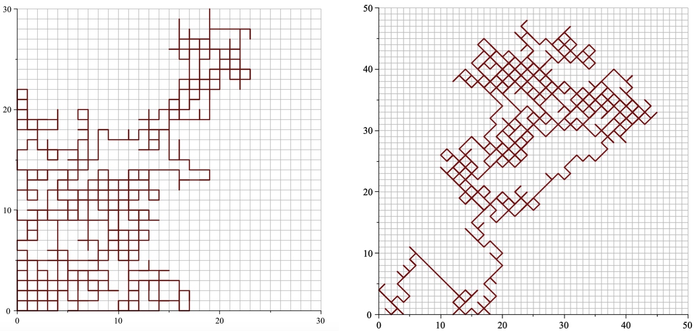
In the unrestricted case, when $\mathcal{R} = \mathbb{R}^d,$ enumeration is straightforward: there are $|\mathcal{S}|$ possibilities for each step, so there are $|\mathcal{S}|^n$ walks of length $n.$ As a consequence, the generating function of an unrestricted walk model is always rational. The generating function of a model restricted to a halfspace $\mathbb{R}_{>0} \times \mathbb{R}^{d-1}$ can be irrational, however a powerful enumerative technique called the kernel method allows one to show that halfspace models always have algebraic generating functions. In contrast, there are two-dimensional walks restricted to the quadrant $\mathbb{R}_{>0}^2$ with generating functions that are transcendental but D-finite, non-D-finite but D-algebraic, and even series that are not D-algebraic (such a series is sometimes called hypertranscendental).

The wide variety of behaviour exhibited by lattice path models even in two dimensions shows that they form an important toolbox to study and develop methods of enumeration. Recent methods developed for the study of quadrant lattice path models have used techniques from computational algebraic geometry, boundary value problems on Riemann surfaces, potential theory, discrete difference equations, differential Galois theory, and complex analysis in several variables.

Advanced Applications of Lattice Paths #

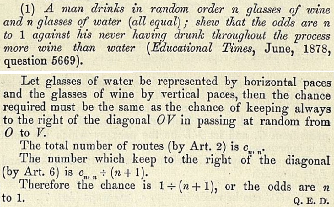
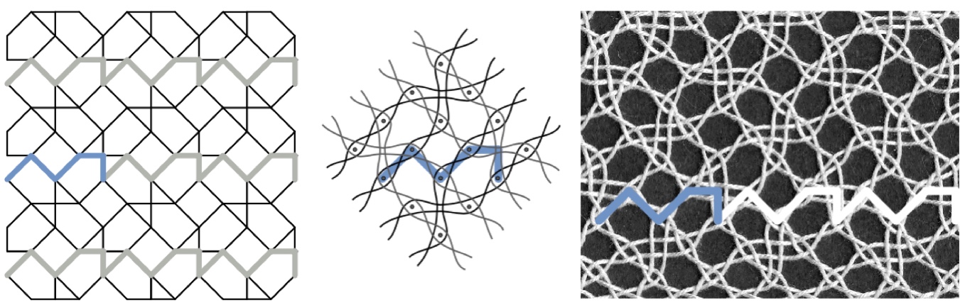
Lattice paths appear frequently in probability theory and the analysis of statistical tests, since a sum of discrete random variables can be interpreted as a random walk. Walks restricted to orthants have many uses in queuing theory, modelling people entering and leaving lines (there can never be a “negative” number of people in line). Further applications include polymer physics, the analysis of data structures, the behaviour of Liouville quantum gravity, the combinatorics of continued fractions, and models for bobbin lace art. Many other combinatorial structures are also naturally encoded by lattice paths.

Integer Compositions and Partitions #

The combinatorial class of (integer) compositions consists of all tuples of positive integers $$ \mathcal{C} = \{(k_1,\dots,k_r) : r, k_j \in \mathbb{N}_{>0} \},$$ where the weight of a tuple $(k_1,\dots,k_r)$ is its sum: $$|(k_1,\dots,k_r)| = k_1 + \cdots + k_r.$$ Thus, the number of objects $c_n$ in $\mathcal{C}$ of weight $n$ is the number of ways to write $n$ as a sum of positive integers where the order of the summands matters. The elements $k_j$ in a composition $(k_1,\dots,k_r) \in \mathcal{C}$ are the parts or summands of the composition, and the number $r$ of elements is the length or number of summands of the composition.

Lemma 1: There are $2^{n-1}$ compositions of size $n.$

By convention, we write a composition $(k_1,\dots,k_r)$ as the sum $k_1 + \cdots + k_r$ of its elements without simplifying.

Example: The compositions of size 3 are $$ 3 = 1 + 1 + 1 = 1 + 2 = 2 + 1.$$

Because Lemma 1 describes the number of compositions of size $n,$ we often enumerate subclasses of compositions defined by various restrictions on the number of summands in the composition or the type of summands that can appear (for instance, asking for the number of compositions of size $n$ with an even number of summands each at most 5).

The class $\mathcal{P}$ of (integer) partitions consists of all non-increasing tuples of positive integers $(k_1,\dots,k_r),$ meaning $k_1 \geq k_2 \geq \cdots \geq k_r.$ Equivalently, partitions are compositions where tuples with the same elements (in a different order) are identified. As for compositions, we usually write partitions as an unsimplified sum.

Example: The partitions of size 3 are $$ 3 = 1 + 1 + 1 = 2 + 1.$$ Note that we no longer include $1 + 2$ as its summands are in increasing order.

The study of partitions is a classical topic in mathematics and combinatorics.

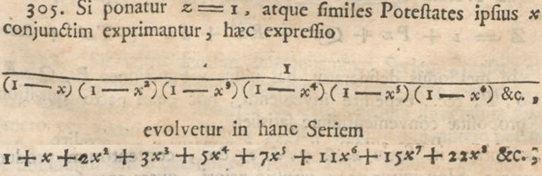
There is no short explicit formula for partitions, but this does not mean they cannot be studied! As far back as the eighteenth century, Euler derived a simple infinite product representation for the generating function of integer partitions, $$ P(z) = \prod_{k \geq 1}\frac{1}{1-z^k}. $$

Similar generating function expressions exist for partitions with various restrictions on the number or type of their summands. The magic of generating functions allows us to, for instance, prove equality between partition families implicitly by manipulating their generating functions. This generating function was also used by Hardy and Ramanujan to derive asymptotics of the number of partitions of size $n$ as $n\rightarrow\infty$ (as mentioned in Chapter 1, a result impressive enough to be a large plot point in a Hollywood movie).

We postpone a full discussion of techniques for partition enumeration until Chapter 9, when partitions will be studied in detail.

Advanced Applications of Compositions and Partitions #

Partitions emerge in the study of physical models, for instance Baxter’s solution of the hard hexagon model used the famous Rogers-Ramanujan identities for the generating functions of certain classes of partitions. Partitions also appear frequently in representation theory — for instance, they index the irreducible representations of the symmetric group and form the signatures of irreducible polynomial representations of the general linear group – and such connections mean that partitions lie at the heart of the geometric complexity theory approach to the P vs NP problem. Combinatorial partition identities also translate to important Lie algebra identities. The enumeration of restricted compositions appeared in the analysis of a post-quantum cryptographic algorithm.

Trees and Graphs #

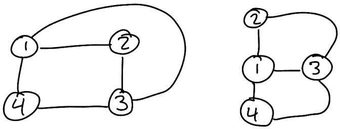
A (finite simple) graph $G$ is a pair of finite sets $G = (V,E)$ where $V$ defines the vertices or nodes of $G$ and $E$ contains the edges of $G,$ which are sets defined by two distinct vertices of $G.$ A graph can be drawn in the plane using circles for the vertices and lines (or curves) between the dots that are connected by edges.

Example: If $G$ is the graph with vertex set $V = \{1,2,3,4\}$ and edge set $E = \{ \{1,2\}, \; \{2,3\}, \; \{3,4\}, \; \{1,3\}, \; \{1,4\} \}$ then two drawings for $G$ are given below.

The study of graphs is an immense area of combinatorics, just as large and perhaps even larger than enumeration, but we restrict ourselves here to summarizing some concepts that will arise in our enumerative journey.

The degree of a vertex is the number of edges it is contained in. A cycle in a graph is a sequence of at least three vertices connected by distinct edges that start and end at the same vertex. For instance, the vertices $1,3,$ and $4$ form a cycle in our last example. A walk in a graph is a sequence of vertices with each consecutive pair in the sequence connected by an edge, and a graph $G$ is connected if for any pair of vertices $a$ and $b$ there is a walk in $G$ starting at $a$ and ending at $b.$

A connected graph with no cycles is called a tree. A rooted graph (usually a rooted tree) is a graph where one vertex, called the root, is specially marked. The height of a vertex $v$ in a rooted tree is one less than the minimal number of vertices in a walk from the root to $v$ (the root itself has height zero). It is common to draw rooted trees with the root on the top, the vertices of height one under the root, the vertices of height two under the vertices of height one, etc. The vertices of height $h+1$ that are connected by an edge to a vertex $v$ of height $h$ are called the children of $v,$ and $v$ is called the parent of these vertices.

A (rooted) $k$-ary tree is a tree where each vertex has $k$ children (which could be empty) and a complete (rooted) $k$-ary tree is a tree where each vertex has either no children or exactly $k$ non-empty children. We often call $2$-ary trees binary trees.

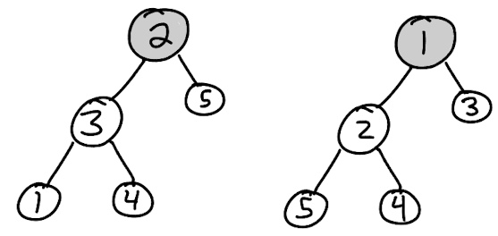
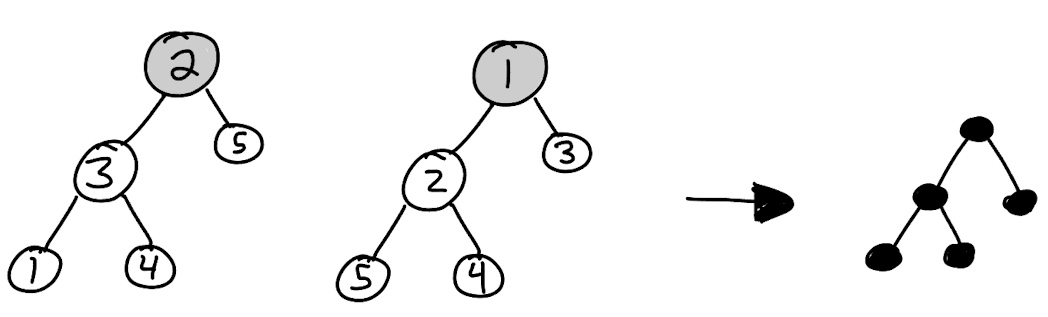
Two graphs $G_1=(V_1,E_1)$ and $G_2=(V_2,E_2)$ are isomorphic if there exists a bijection $f:V_1\rightarrow V_2$ such that any pair of distinct vertices $a$ and $b$ form an edge in $E_1$ if and only if the images $f(a)$ and $f(b)$ form an edge in $E_2.$ Rooted graphs are isomorphic when there is an isomorphism that sends the root in one graph to the root of another.

A labelled graph class is a combinatorial class defined by a set $\mathcal{G}$ of graphs with vertex sets of the form $V = [n]$ for $n\in\mathbb{N}$ together with a weight function, typically taken as the number of vertices, although other common weightings include number of edges or number of vertices of degree one (when this does define a combinatorial class). An unlabelled graph class is a combinatorial class defined by a set $\mathcal{G}$ of graphs with vertex sets of the form $V = [n]$ for $n\in\mathbb{N}$ where isomorphic graphs are identified, together with an appropriate weight function.

Lemma 2: There are $2^{\binom{n}{2}}$ labelled graphs with $n$ vertices.

Remark: Recall from Chapter 1 that it is an open problem whether the number of unlabelled graphs on $n$ vertices can be computed in polynomial time with respect to $n.$

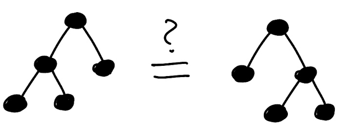
Finally, we note that we can view graphs both as abstract structures and as drawings of those structures in the plane. This comes up for us in the enumeration of different kinds of trees. A class of rooted trees is called planar if the order of the children of each node matters (i.e., must be respected when considering two graphs isomorphic) and non-planar if the order of the children does not matter.

Remark: The term planar comes from the fact that planar trees rely on their embedding in the plane. Do not confuse this with the other meaning of planar in graph theory (that the graph can be drawn in the plane with no edges crossing – every tree can be drawn in the plane with no edges crossing). The distinction of planar and non-planar graphs is only interesting in the unlabelled case, because in the labelled case every node is unique.

Advanced Applications #

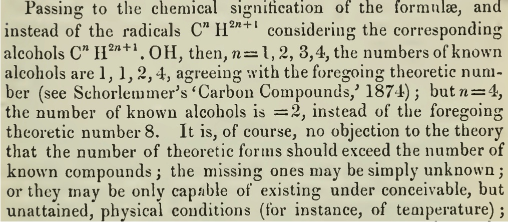
Graphs are embedded into the foundations of modern computer science, so it comes as no surprise that the combinatorial study of trees and graphs is key to many crucial results in the analysis of algorithms and data structures. A small selection of the many other interesting applications of graphs include phylogenetic trees used in evolutionary models, graph algorithms as primitives for quantum computing, the analysis of social networks and internet routing, and the use of graphs to model chemical isomers (for instance, in 1875 Cayley used a graph theoretic analysis to argue that there should be eight pentanol isomers, even though only 2 were known at the time – now it is known that all eight isomers do exist).