Nowhere more than in combinatorial theory do we see the fallacy of Kronecker’s well-known saying that “God created the integers; everything else is man-made.” A more accurate description might be: “God created infinity, and man, unable to understand infinity, had to invent finite sets.” In the ever-present interaction of finite and infinite lies the fascination of all things combinatorial.
— Gian-Carlo Rota
It is the mark of an educated mind... not to seek exactness where only an approximation is possible.
— Aristotle
Our study of the large-scale behaviour of objects now brings us to the topic of asymptotics. Roughly speaking, even complicated sequences are often well-approximated by simple ones as their indices $n$ grow large, and such an approximation allows for a clear understanding of how the sequence behaves (including capturing the behaviour of sequences that don’t admit nice closed forms).
To discuss asymptotics rigorously we need to define how we compare sequences.
A sequence $p_n$ is called eventually positive if there exists some $N \in \mathbb{N}$ such that $p_n > 0$ for all $n \geq N.$ Let $f_n$ and $g_n$ be two eventually positive sequences (typically $f_n$ is a complicated expression and $g_n$ is a simpler expression it is being compared to).
We write $f_n \sim g_n$ and say that $f_n$ is asymptotic to $g_n$ if
$$\lim_{n \rightarrow\infty} \frac{f_n}{g_n} = 1.$$
If $f_n \sim g_n$ then $f_n$ grows “approximately like” $g_n.$
Example: If $f_n=n^2+ 1000n - 17$ and $g_n = n^2$ then $f_n \sim g_n$ since
$$ \lim_{n \rightarrow\infty} \frac{f_n}{g_n} = \lim_{n \rightarrow\infty} \frac{n^2+ 1000n - 17}{n^2} = \lim_{n \rightarrow\infty}\left(1 + \frac{1000}{n} - \frac{17}{n^2}\right)=1.$$
We write $f_n = O(g_n)$ and say that $f_n$ is big-O of $g_n$ if there exist $C>0$ and $N \in \mathbb{N}$ such that
$$ f_n \leq C \cdot g_n \text{ for all $n \geq N$} $$
If $f_n=O(g_n)$ then $f_n$ grows “at most like” a constant times $g_n.$
Example: If $f_n=n^2 + 1000n - 17$ and $g_n = 2n^2$ then $f_n = O(g_n)$ since
$$ f_n \leq g_n \text{ for all } n \geq 1000 $$
because $1000n - 17 \leq n^2$ when $n \geq 1000.$
Example: If $f_n=2n^2 + n$ and $g_n = n^2$ then $f_n = O(g_n)$ since
$$ f_n \leq 3g_n \text{ for all } n \geq 3 $$
Note that $f_n$ is larger than $g_n$ for all $n,$ but only by a constant factor.
Note: We often use the term $O(g_n)$ to denote a set of sequences, so it is technically more proper to write $f_n \in O(g_n)$ instead of $f_n = O(g_n).$ However, the notation $f_n = O(g_n)$ is useful and more widely used, so we adopt it here.
We write $f_n = o(g_n)$ and say that $f_n$ is little-O of $g_n$ if
$$\lim_{n \rightarrow\infty} \frac{f_n}{g_n} = 0$$
If $f_n=o(g_n)$ then $f_n$ grows “slower than” a constant times $g_n.$
Example: If $f_n=n^2 + 1000n - 17$ and $g_n = n^3$ then $f_n = o(g_n)$ since
$$\lim_{n \rightarrow\infty} \frac{f_n}{g_n} = \lim_{n \rightarrow\infty} \frac{n^2+ 1000n - 17}{n^3} = \lim_{n \rightarrow\infty}\left(\frac{1}{n} + \frac{1000}{n^2} - \frac{17}{n^3}\right)=0.$$
Example: A sequence $f_n = o(1)$ if and only if $f_n \rightarrow 0$ as $n\rightarrow\infty.$
Note: All of these definitions depend only on the limit behaviour of $f_n$ and $g_n$ as $n\rightarrow\infty,$ so changing any finite number of terms in $f_n$ or $g_n$ does not change whether $f_n$ is asymptotic to (or big/little-O of) $g_n.$ In particular, since $f_n$ and $g_n$ are eventually positive we can assume in proofs that our sequences contain only positive terms (if needed).
We also recall some more advanced examples from Chapter 1.
Example: Although it has been an open problem since the 1980s whether the number $g_n$ of (unlabelled) graphs on $n$ vertices can be computed in polynomial time, the asymptotic behaviour
$$ g_n \sim \frac{2^{\binom{2n}{n}}}{n!} $$
follows from classical probabilistic work of Erdős and Rényi in the 1960s.
Example: If $p_n$ denotes the number of integer partitions of size $n$ then Hardy and Ramanujan derived the asymptotic formula
$$ p_n \sim \frac{\exp\left(\pi\sqrt{2n/3}\right)}{4n\sqrt{3}} $$
using advanced analytic techniques. There is technically an explicit formula for $p_n,$ but it took hundreds of years to discover and is extremely unwieldy.
We begin by showing that we can use asymptotic notation algebraically. For simplicity, given sequences $(f_n)$ and $(g_n)$ we write $f_n + g_n$ to denote the sequence obtained from $f_n$ and $g_n$ by term-wise addition, and $f_ng_n$ to denote the sequence obtained by term-wise multiplication.
Lemma 1: Let $f_n,g_n,a_n,b_n$ be eventually positive sequences.
If $f_n = O(a_n)$ and $g_n = O(b_n)$ then
$$f_n + g_n = O(a_n + b_n) \text{ and } f_n g_n = O(a_n b_n).$$
If $f_n = o(a_n)$ and $g_n = o(b_n)$ then
$$f_n + g_n = o(a_n + b_n) \text{ and } f_n g_n = o(a_n b_n).$$
Proof of Lemma 1
As noted above, we can assume without loss of generality that all sequences contain positive terms.
(Big-O) We know there exist constants $C_1,C_2,N_1,N_2>0$ such that
$$ f_n \leq C_1 a_n \text{ for all } n \geq N_1$$
and
$$ g_n \leq C_2 b_n \text{ for all } n \geq N_2.$$
Thus,
$$ f_n + g_n \leq C_3(a_n+b_n) \text{ for all } n \geq N_3,$$
where $C_3 = \max(C_1,C_2)$ and $N_3 = \max(N_1,N_2),$ so $f_n + g_n = O(a_n+b_n).$
(Little-O) Analogous to big-O.
Algebraic equations involving big-O notation can be interpreted using sequences taken from each of the big-O terms (and the same for little-O). For instance, we write $a_n = b_n + O(g_n)$ if there exists a function $c_n = O(g_n)$ such that $a_n = b_n + c_n$ (recall the discussion above about using equality instead of set membership in big-O notation).
Lemma 2: Let $f_n,g_n,a_n,b_n$ be eventually positive sequences. Then
(a) $f_n = g_n(1+o(1))$ if and only if $f_n \sim g_n$
(b) If $f_n = a_n + b_n$ with $a_n \sim g_n$ and $b_n = o(g_n)$ then $f_n \sim g_n$
Proof of Lemma 2
(a) By definition
$$
\begin{aligned}
f_n \sim g_n &\leftrightarrow
f_n/g_n \text{ goes to $1$ as $n\rightarrow\infty$} \\
&\leftrightarrow f_n/g_n = 1 + c_n \text{ for some sequence $c_n \rightarrow0$ as $n\rightarrow\infty$}
\\
&\leftrightarrow f_n = g_n(1+c_n) \text{ where } c_n = o(1).
\end{aligned}
$$
(b) We have
$$ \lim_{n \rightarrow\infty} \frac{f_n}{g_n} = \lim_{n \rightarrow\infty} \frac{a_n + b_n}{g_n} = \lim_{n \rightarrow\infty} \frac{a_n}{g_n} + \lim_{n \rightarrow\infty} \frac{b_n}{g_n} = 1 + 0 =1,$$
as desired.
Note: The notation $f_n \sim g_n$ makes sense for any complex-valued sequences $f_n$ and $g_n,$ as long as $g_n \neq 0$ for all sufficiently large $n$ so the ratio $f_n/g_n$ is defined. We reserve big-O and little-O notation only for eventually positive sequences because they represent upper bounds, however an arbitrary complex-valued sequence $f_n$ gives rise to bounds $O(|f_n|)$ and $o(|f_n|).$
Most of the asymptotic forms we discuss are made up of sequences coming from a few basic families.
Family Name
General Member
Example
constants
$f_n = A$ for some $A>0$
$f_n = 1$
log-powers
$f_n = (\log n)^B$ for some $B>0$
$f_n = \sqrt{\log n}$
powers of $n$
$f_n = n^C$ for some $C>0$
$f_n = n^{1/3}$
exponentials
$f_n = D^n$ for some $D>1$
$f_n = 2^n$
$n^n$ powers
$f_n = n^{En}$ for some $E>0$
$f_n = n^{2n}$
Other types of sequences also arise in asymptotic results – for instance, in the simple graph and partition examples above – but the majority of examples we encounter have nice closed forms involving these expressions.
Lemma 3: The families listed above form an asymptotic hierarchy: any constant is little-o of any log-power, which is little-o of any power of $n,$ which is little-o of any exponential, which is little-o of any $n^n$ power.
Thus, if we have two sequences and want to know which is asymptotically bigger, first we compare any $n^n$-powers, then compare any exponentials, then compare any powers of $n,$ etc.
We prove each level of the hierarchy in order. Because asymptotic behaviour is a limiting process, basic tools from calculus are useful in asymptotic arguments.
$A = o((\log n)^B)$ when $B>0$ since
$$\lim_{n \rightarrow\infty} \frac{A}{(\log n)^B} = 0.$$
When $C,B>0$ then
$$
\begin{aligned}
\lim_{n \rightarrow\infty} \frac{(\log n)^B}{n^C}
&= \left(\lim_{n \rightarrow\infty} \frac{\log n}{n^{C/B}} \right)^B \\[+3mm]
&= \left(\lim_{n \rightarrow\infty} \frac{1/n}{(C/B)n^{C/B-1}} \right)^B \\[+3mm]
&= \left(\lim_{n \rightarrow\infty} \frac{B/C}{n^{C/B}} \right)^B \\[+3mm]
&= 0,
\end{aligned}
$$
where the first equality follows from the fact that the function $f(x)=x^B$ is continuous and the second equality follows from L’Hôpital’s Rule.
Let $M = \lceil C \rceil.$ Applying L’Hôpital’s Rule $M$ times gives
$$ \lim_{n\rightarrow\infty} \frac{n^M}{D^n} = \lim_{n\rightarrow\infty} \frac{M!}{(\log D)^M} \cdot D^{-n} = 0.$$
Since $\displaystyle 0 \leq \frac{n^C}{D^n} \leq \frac{n^M}{D^n},$ the squeeze theorem implies $\lim_{n\rightarrow\infty} \frac{n^C}{D^n}=0.$
By continuity,
$$ \lim_{n \rightarrow\infty} \frac{D^n}{n^{En}} = \lim_{n \rightarrow\infty} \left(\frac{D}{n^E}\right)^n.$$
For $n$ sufficiently large $\displaystyle\frac{D}{n^E} < 1/2,$ so
$$ 0 \leq \lim_{n \rightarrow\infty} \frac{D^n}{n^{En}} \leq \lim_{n\rightarrow\infty}\left(\frac{1}{2}\right)^n$$
and thus $\displaystyle\lim_{n \rightarrow\infty} \frac{D^n}{n^{En}} = 0.$
The families chosen above reflect the fact that the sequences we consider typically grow to infinity as $n\rightarrow\infty.$ A reverse result holds for the reciprocals of these families, which approach zero as $n\rightarrow\infty.$
Exercise: Prove that the following families of sequences form an asymptotic hierarchy, in the sense of Lemma 3.
We have seen above that derivatives are useful in asymptotic arguments via L’Hôpital’s Rule (Taylor series are also very useful for asymptotic approximations). Similarly, because integrals are defined as limits of sums, integration can be useful for determining the asymptotic behaviour of series.
Example: The arithmetic series
$$\sum_{k=1}^n k = \frac{n(n+1)}{2} \sim \frac{n^2}{2}.$$
What can we say about the sum $\displaystyle s_n = \sum_{k=1}^n k^2$ as $n\rightarrow\infty$?
Although $s_n$ can be determined exactly as a polynomial in $n,$ we focus on an asymptotic method that generalizes to a broader class of sequences. In particular, we approximate $s_n$ by an integral using Riemann sums.
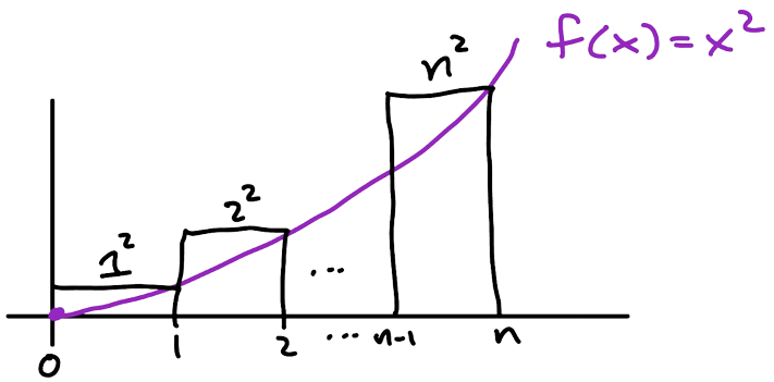
If $f(x) = x^2$ then we can take a “right-hand Riemann sum” and see that
$$ \int_0^n x^2 dx \leq \sum_{k=1}^n k^2$$
by comparing the area covered by a finite number of rectangles with widths 1 and heights $f(1),f(2),\dots,f(n)$ to an area under the curve $f(x).$
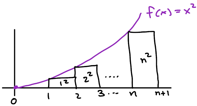
Similarly, shifting our domain of integration, we can take a “left-hand Riemann sum” and see that
$$ \sum_{k=1}^n k^2 \leq \int_1^{n+1} x^2 dx$$
by comparing the area covered by a finite number of rectangles with an area under the curve $f(x).$
Putting these two results together, and using the antiderivative $\int x^2 dx = x^3/3,$ gives
$$ \frac{n^3}{3} \leq \sum_{k=1}^n k^2 \leq \frac{(n+1)^3}{3} - 1 $$
so $\displaystyle \sum_{k=1}^n k^2 \sim \frac{n^3}{3}. $
Note: Although sums are “simpler” objects, integrals are usually easier to compute in closed form (a miracle of calculus).
The approach in this last example can be greatly generalized.
Theorem: Let $a<b$ be integers and let $f(x)$ be a continuous function on the interval $[a-1,b+1].$
(a) If $f$ is increasing on $[a-1,b+1]$ then
$$ \int_{a-1}^b f(x) dx \leq \sum_{k=a}^b f(k) \leq \int_a^{b+1}f(x)dx.$$
(b) If $f$ is decreasing on $[a-1,b+1]$ then
$$ \int_{a-1}^b f(x) dx \geq \sum_{k=a}^b f(k) \geq \int_a^{b+1}f(x)dx.$$
Exercise: Follow the argument in the last to example to prove this theorem.
Corollary: Let $a<b$ be integers and $f(x)$ be a continuous function on $I = [a-1,b+1].$ If $f$ is either decreasing on $I$ or increasing on $I,$ and $|f(x)| \leq M$ on $I,$ then
$$ \left|\sum_{k=a}^b f(k) - \int_a^b f(x) dx \right| \leq M. $$
Proof of Corollary
The upper and lower bounds on $\sum_{k=a}^b f(k)$ in the last theorem differ by an integral of $f(x)$ over an interval of length one, and since $f$ is continuous
$$ \left| \int_J f(x) dx \right| \leq \text{length}(J) \cdot \max_{x \in J} |f(x)|$$
for any interval $J.$
Example: Let $\alpha>0.$ Since the function $f(x) = x^\alpha$ has $f^\prime(x) = \alpha x^{\alpha-1}>0$ for any $x>0$ we see that $f$ is increasing and the Corollary implies
$$ \sum_{k=1}^n k^\alpha = \frac{n^{\alpha+1}}{\alpha+1} + O(n^\alpha). $$
Note that this not only applies to positive integer $\alpha$ (when an exact but cumbersome expression for the sum as a polynomial in $n$ can always be determined) but also to non-integer $\alpha$ (when no such explicit expressions may exist).
Our next example comes up in the analysis of many combinatorial objects (for instance, it already arose as the average number of cycles among the permutations of length $n$).
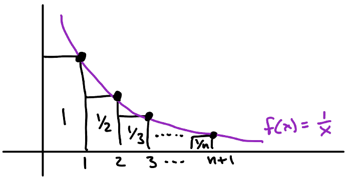
Example: Find the asymptotic behaviour of the Harmonic number $H_n = \sum_{k=1}^n \frac{1}{k}.$
Click for Answer
Because $f(x) = 1/x$ is decreasing for $x>0$ we see that
$$ H_n \geq \int_1^{n+1}\frac{dx}{x} = \log(n+1).$$
Since $f(x)$ is not defined at $x=0,$ we take out the first term of the sum and bound
$$H_n-1 = \sum_{k=2}^n\frac{1}{k} \leq \int_1^n \frac{dx}{x} = \log n.$$
Thus,
$$ \log n < \log(n+1) \leq H_n \leq \log n + 1 $$
so $H_n \sim \log n.$
A sorting algorithm takes a tuple of unique comparable objects and returns a new tuple with the same objects listed in increasing order. Sorting algorithms are typically classified by how many comparisons they make when sorting tuples of $n$ elements, as a function of $n$ (more advanced analyses take into account things like the cost to access elements in memory, cache misses, and other practical details that we abstract away).
Because we track only the number of comparisons, the elements themselves are irrelevant — we only need them to be distinct and comparable. Thus, to study the complexity of a sorting algorithm we may assume that it takes as input a permutation and track how many pairs of elements are compared in order to swap back to the identity permutation.
Example: Consider the selection sort algorithm which sorts a permutation $\pi$ by building a list of sorted elements iteratively starting at the first position.
selection_sort(pi):
for i from1 to n:
m = i
for j from i+1 to n:
if pi(j) < m: # pi(j) = jth element of pi m = j
# m is now the index of ith smallest element# put ith smallest element in correct place then move on swap pi(i) and pi(m)
For any permutation of size $n,$ selection sort does a comparison of elements for every pair $(i,j)$ of natural numbers with $i \in \{1,\dots,n\}$ and $j \in \{i+1,\dots,n\}.$ Thus, selection sort always performs
$$ \sum_{i=1}^n (n-i) = \sum_{i=0}^{n-1} i = \frac{n(n-1)}{2} \sim \frac{n^2}{2} $$
comparisons when given a permutation of size $n.$
In general, sorting algorithms make a different number of comparisons depending on the permutation inputted (not just its size) and are commonly ranked by one of two measures: the worst-case maximum number of comparisons among all permutations of size $n,$ or the average number of comparisons over all permutations of size $n.$
One of the most important, and most used, sorting algorithms in computer science is quicksort. At a high level, quicksort sorts a tuple $\pi$ by
picking a random element of $\pi$ (called a pivot)
going through $\pi$ and moving everything less than the pivot to its left, and everything greater than the pivot to its right
recursively sorting the elements to the left and right of the pivot.
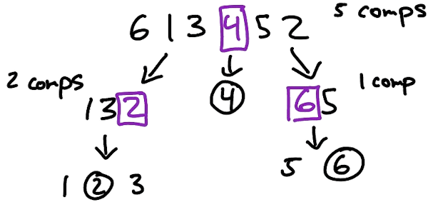
Figure:
A run of quicksort on a permutation of size 6, using 8 comparisons.
In the worst case the pivot selected at each recursive step is the highest or lowest element, in which case recursive calls of size $n-1,n-2,\dots,2$ are made and a total of
$$ \sum_{i=1}^{n-1} i = \frac{n(n-1)}{2} \sim \frac{n^2}{2} $$
comparisons are made. But what about the average case?
Let $c_n$ be the average number of comparisons quicksort does over all permutations of size $n.$ Then $c_0=c_1=0$ and for $n>1$ we have
$$ c_n = \frac{1}{n} \sum_{k=1}^n {\Big[}(n-1) + c_{k-1} + c_{n-k} {\Big]},$$
where for each possible value $k$ of the pivot,
$n-1$ tracks the comparisons made on input of size $n$ before a recursive call,
$c_{k-1}$ tracks the comparisons made on the elements to the left of the pivot,
$c_{n-k}$ tracks the comparisons made on the elements to the right of the pivot,
and the leading factor of $1/n$ averages over all values of the pivot.
Algebraic manipulation implies
$$ c_n = (n-1) + \frac{1}{n} \left[ \sum_{k=1}^nc_{k-1} + \sum_{k=1}^n c_{n-k} \right] = (n-1) + \frac{2}{n}\sum_{k=1}^{n-1} c_k $$
for all $n \geq 1,$ so
$$nc_n = (n-1)n + 2 \sum_{k=1}^{n-1} c_k .$$
Substituting $n \rightarrow n-1$ gives
$$(n-1)c_{n-1} = (n-2)(n-1) + 2 \sum_{k=1}^{n-2} c_k $$
and subtracting these last two equations implies, after some algebraic manipulation, that
$$nc_n = (n+1)c_{n-1} + 2(n-1)$$
for all $n \geq 1.$ Thus,
$$
\begin{aligned}
\frac{c_n}{n+1} &= \frac{c_{n-1}}{n} + \frac{2}{n+1} - \frac{2}{n(n+1)} \\[+4mm]
&\leq \frac{c_{n-1}}{n} + \frac{2}{n+1} \\[+4mm]
&\leq \frac{c_{n-2}}{n-1} + \frac{2}{n} - \frac{2}{(n-1)n} + \frac{2}{n+1} \\[+2mm]
&\leq \frac{c_{n-2}}{n-1} + \frac{2}{n} + \frac{2}{n+1} \\[+2mm]
& \;\; \vdots \\
&\leq \frac{c_1}{2} + \sum_{k=2}^n \frac{2}{k+1} \\[+4mm]
&= 2 \sum_{k=2}^n \frac{1}{k+1}.
\end{aligned}
$$
The arguments above imply
$$ \sum_{k=2}^n \frac{1}{k+1} \leq \int_1^n \frac{dx}{1+x} = \log (n+1) - \log(2),$$
so the average number of comparisons performed by quicksort on an input of size $n$ is $c_n \leq 2(n+1)\log(n+1) = O(n\log n).$
Exercise:(a) Multiply both sides of the linear recurrence
$$nc_n = (n+1)c_{n-1} + 2(n-1)$$
by $z^n$ and sum the result to prove that the generating function $C(z)$ of $c_n$ satisfies the linear differential equation
$$ (1-z)^3C^\prime(z) - 2(1-z)^2C(z) - 2z = 0.$$
(b) Solve this first order differential equation (using a computer algebra system if necessary) to prove that
$$ C(z) = \frac{-2\log(1-z)}{(1-z)^2} - \frac{2z}{(1-z)^2}. $$
(c) Prove that
$$[z^n]\frac{-\log(1-z)}{(1-z)^2} = (n+1)H_n - n$$
where $H_n$ is the $n$th Harmonic number, and then show that
$$ c_n = 2(n+1)H_n - 4n \sim 2n\log n.$$
Note that the best-case number of comparisons occurs when the pivot is chosen to be in the middle of the elements in each step, which gives $n \log_2 n$ comparisons. Since $2n\log n \approx 1.39n \log_2n$ we see that the average performance of quicksort is approximately 39% worse than the best case. This explains why quicksort is quick in practice, even though its worse case number of comparisons is quadratic in the size of the input.